Survival analysis
This notebook presents example usage of package for solving survival problem on bmt dataset. You can access dataset here
This tutorial will cover topics such as:
- training model
- changing model hyperparameters
- hyperparameters tuning
- calculating metrics for model
Install dependencies
[ ]:
%pip install matplotlib
Summary of the dataset
[ ]:
import pandas as pd
import numpy as np
from rulekit.arff import read_arff

DATASET_URL: str = (
    'https://raw.githubusercontent.com/'
    'adaa-polsl/RuleKit/master/data/bmt/'
    'bmt.arff'
)
data_df: pd.DataFrame = read_arff(DATASET_URL)
data_df['survival_status'] = data_df['survival_status'].astype(int).astype(str)
data_df
| Recipientgender | Stemcellsource | Donorage | Donorage35 | IIIV | Gendermatch | DonorABO | RecipientABO | RecipientRh | ABOmatch | ... | extcGvHD | CD34kgx10d6 | CD3dCD34 | CD3dkgx10d8 | Rbodymass | ANCrecovery | PLTrecovery | time_to_aGvHD_III_IV | survival_time | survival_status | |
|---|---|---|---|---|---|---|---|---|---|---|---|---|---|---|---|---|---|---|---|---|---|
| 0 | 1 | 1 | 22.830137 | 0 | 1 | 0 | 1 | 1 | 1 | 0 | ... | 1 | 7.20 | 1.338760 | 5.38 | 35.0 | 19.0 | 51.0 | 32.0 | 999.0 | 0 |
| 1 | 1 | 0 | 23.342466 | 0 | 1 | 0 | -1 | -1 | 1 | 0 | ... | 1 | 4.50 | 11.078295 | 0.41 | 20.6 | 16.0 | 37.0 | 1000000.0 | 163.0 | 1 |
| 2 | 1 | 0 | 26.394521 | 0 | 1 | 0 | -1 | -1 | 1 | 0 | ... | 1 | 7.94 | 19.013230 | 0.42 | 23.4 | 23.0 | 20.0 | 1000000.0 | 435.0 | 1 |
| 3 | 0 | 0 | 39.684932 | 1 | 1 | 0 | 1 | 2 | 1 | 1 | ... | None | 4.25 | 29.481647 | 0.14 | 50.0 | 23.0 | 29.0 | 19.0 | 53.0 | 1 |
| 4 | 0 | 1 | 33.358904 | 0 | 0 | 0 | 1 | 2 | 0 | 1 | ... | 1 | 51.85 | 3.972255 | 13.05 | 9.0 | 14.0 | 14.0 | 1000000.0 | 2043.0 | 0 |
| ... | ... | ... | ... | ... | ... | ... | ... | ... | ... | ... | ... | ... | ... | ... | ... | ... | ... | ... | ... | ... | ... |
| 182 | 1 | 1 | 37.575342 | 1 | 1 | 0 | 1 | 1 | 0 | 0 | ... | 1 | 11.08 | 2.522750 | 4.39 | 44.0 | 15.0 | 22.0 | 16.0 | 385.0 | 1 |
| 183 | 0 | 1 | 22.895890 | 0 | 0 | 0 | 1 | 0 | 1 | 1 | ... | 1 | 4.64 | 1.038858 | 4.47 | 44.5 | 12.0 | 30.0 | 1000000.0 | 634.0 | 1 |
| 184 | 0 | 1 | 27.347945 | 0 | 1 | 0 | 1 | -1 | 1 | 1 | ... | 1 | 7.73 | 1.635559 | 4.73 | 33.0 | 16.0 | 16.0 | 1000000.0 | 1895.0 | 0 |
| 185 | 1 | 1 | 27.780822 | 0 | 1 | 0 | 1 | 0 | 1 | 1 | ... | 0 | 15.41 | 8.077770 | 1.91 | 24.0 | 13.0 | 14.0 | 54.0 | 382.0 | 1 |
| 186 | 1 | 1 | 55.553425 | 1 | 1 | 0 | 1 | 2 | 1 | 1 | ... | 1 | 9.91 | 0.948135 | 10.45 | 37.0 | 18.0 | 20.0 | 1000000.0 | 1109.0 | 0 |
187 rows × 37 columns
[3]:
print("Dataset overview:")
print(f"Name: bmt")
print(f"Objects number: {data_df.shape[0]}; Attributes number: {data_df.shape[1]}")
print("Basic attribute statistics:")
data_df.describe()
Dataset overview:
Name: bmt
Objects number: 187; Attributes number: 37
Basic attribute statistics:
[3]:
| Donorage | Recipientage | CD34kgx10d6 | CD3dCD34 | CD3dkgx10d8 | Rbodymass | ANCrecovery | PLTrecovery | time_to_aGvHD_III_IV | survival_time | |
|---|---|---|---|---|---|---|---|---|---|---|
| count | 187.000000 | 187.000000 | 187.000000 | 182.000000 | 182.000000 | 185.000000 | 187.000000 | 187.000000 | 187.000000 | 187.000000 |
| mean | 33.472068 | 9.931551 | 11.891781 | 5.385096 | 4.745714 | 35.801081 | 26752.866310 | 90937.919786 | 775408.042781 | 938.743316 |
| std | 8.271826 | 5.305639 | 9.914386 | 9.598716 | 3.859128 | 19.650922 | 161747.200525 | 288242.407688 | 418425.252689 | 849.589495 |
| min | 18.646575 | 0.600000 | 0.790000 | 0.204132 | 0.040000 | 6.000000 | 9.000000 | 9.000000 | 10.000000 | 6.000000 |
| 25% | 27.039726 | 5.050000 | 5.350000 | 1.786683 | 1.687500 | 19.000000 | 13.000000 | 16.000000 | 1000000.000000 | 168.500000 |
| 50% | 33.550685 | 9.600000 | 9.720000 | 2.734462 | 4.325000 | 33.000000 | 15.000000 | 21.000000 | 1000000.000000 | 676.000000 |
| 75% | 40.117809 | 14.050000 | 15.415000 | 5.823565 | 6.785000 | 50.600000 | 17.000000 | 37.000000 | 1000000.000000 | 1604.000000 |
| max | 55.553425 | 20.200000 | 57.780000 | 99.560970 | 20.020000 | 103.400000 | 1000000.000000 | 1000000.000000 | 1000000.000000 | 3364.000000 |
Helper function for creating ruleset characteristics dataframe
[4]:
def get_ruleset_stats(model) -> pd.DataFrame:
    tmp = model.parameters.__dict__
    del tmp['_java_object']
    return pd.DataFrame.from_records([{**tmp, **model.stats.__dict__}])
Rule induction on full dataset
[5]:
X: pd.DataFrame = data_df.drop(['survival_status'], axis=1)
y: pd.Series = data_df['survival_status']
[6]:
from rulekit.survival import SurvivalRules
from rulekit.rules import RuleSet, SurvivalRule

srv = SurvivalRules(survival_time_attr='survival_time')

srv.fit(X, y)

ruleset: RuleSet[SurvivalRule] = srv.model

predictions: np.ndarray = srv.predict(X)


ruleset_stats = get_ruleset_stats(ruleset)


display(ruleset_stats)
| minimum_covered | maximum_uncovered_fraction | ignore_missing | pruning_enabled | max_growing_condition | time_total_s | time_growing_s | time_pruning_s | rules_count | conditions_per_rule | induced_conditions_per_rule | avg_rule_coverage | avg_rule_precision | avg_rule_quality | pvalue | FDR_pvalue | FWER_pvalue | fraction_significant | fraction_FDR_significant | fraction_FWER_significant | |
|---|---|---|---|---|---|---|---|---|---|---|---|---|---|---|---|---|---|---|---|---|
| 0 | 0.05 | 0.0 | False | True | 0.0 | 1.771417 | 0.797513 | 0.902853 | 5 | 3.6 | 65.2 | 0.308021 | 1.0 | 0.999865 | 0.000135 | 0.000147 | 0.000184 | 1.0 | 1.0 | 1.0 |
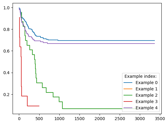
Plot predicted estimators for the first five examples
[7]:
import matplotlib.pyplot as plt

for i in range(5):
    plt.step(
        predictions[i]["times"],
        predictions[i]["probabilities"],
        label=f'Example {i}'
    )
plt.legend(title='Example index:')
[7]:
<matplotlib.legend.Legend at 0x289deb3a180>
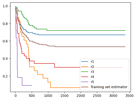
Plot rules Kaplan-Meier’s estimators on top of the training dataset estimator
[8]:
from rulekit.kaplan_meier import KaplanMeierEstimator

# plot rules kaplan-meier curves
for i, rule in enumerate(ruleset.rules):
    rule_label: str = f'r{i + 1}'
    rule_km: KaplanMeierEstimator = rule.kaplan_meier_estimator
    plt.step(
        rule_km.times,
        rule_km.probabilities,
        label=rule_label
    )
    print(f'{rule_label}: {rule}')

# plot whole dataset kaplan-meier curve
train_km: KaplanMeierEstimator = srv.get_train_set_kaplan_meier()
plt.step(
    train_km.times,
    train_km.probabilities,
    label='Training set estimator'
)

plt.legend()
plt.show()
r1: IF Donorage = (-inf, 45.16) AND Relapse = {0} AND Recipientage = (-inf, 17.45) THEN
r2: IF Donorage = (-inf, 43.63) AND HLAmismatch = {0} AND Relapse = {1} THEN
r3: IF PLTrecovery = (-inf, 266) AND time_to_aGvHD_III_IV = <12.50, inf) AND ANCrecovery = <10.50, 19.50) AND Rbodymass = (-inf, 69) AND Donorage = (-inf, 44.06) AND Recipientage = <4.60, inf) AND CD34kgx10d6 = (-inf, 16.98) THEN
r4: IF Donorage = <37.16, inf) AND Recipientage = <5.15, inf) AND time_to_aGvHD_III_IV = <23.50, inf) AND CD3dCD34 = <0.90, 73.72) THEN
r5: IF Recipientage = <17.85, 18.85) THEN
Rules evaluation on full set
[9]:
integrated_brier_score = srv.score(X, y)
print(f'Integrated Brier Score: {integrated_brier_score}')
Integrated Brier Score: 0.19651358709002972
Stratified K-Folds cross-validation
[10]:
from sklearn.model_selection import StratifiedKFold
from rulekit.exceptions import RuleKitJavaException

skf = StratifiedKFold(n_splits=10, shuffle=True, random_state=0)

ruleset_stats = pd.DataFrame()
survival_metrics = []

for train_index, test_index in skf.split(X, y):
    X_train, X_test = X.iloc[train_index], X.iloc[test_index]
    y_train, y_test = y.iloc[train_index], y.iloc[test_index]

    srv = SurvivalRules(
        survival_time_attr='survival_time'
    )
    srv.fit(X_train, y_train)

    ruleset = srv.model

    ibs: float = srv.score(X_test, y_test)

    survival_metrics.append(ibs)
    ruleset_stats = pd.concat([ruleset_stats, get_ruleset_stats(ruleset)])
Ruleset characteristics (average)
[11]:
display(ruleset_stats.mean())
minimum_covered                 0.050000
maximum_uncovered_fraction      0.000000
ignore_missing                  0.000000
pruning_enabled                 1.000000
max_growing_condition           0.000000
time_total_s                    0.799019
time_growing_s                  0.296248
time_pruning_s                  0.477474
rules_count                     4.000000
conditions_per_rule             2.581667
induced_conditions_per_rule    59.825000
avg_rule_coverage               0.486613
avg_rule_precision              1.000000
avg_rule_quality                0.995955
pvalue                          0.004045
FDR_pvalue                      0.004061
FWER_pvalue                     0.004104
fraction_significant            0.980000
fraction_FDR_significant        0.980000
fraction_FWER_significant       0.980000
dtype: float64
Rules evaluation on dataset (average)
[12]:
print(f'Integrated Brier Score: {np.mean(survival_metrics)}')
Integrated Brier Score: 0.20178456199764142
Hyperparameters tuning
This one gonna take a while…
[13]:
from sklearn.model_selection import StratifiedKFold
from sklearn.model_selection import GridSearchCV
[14]:
def scorer(estimator: SurvivalRules, X: pd.DataFrame, y: pd.Series) -> float:
    return -1 * estimator.score(X, y)
[18]:
# define models and parameters
model = SurvivalRules(survival_time_attr='survival_time')

# define grid search
grid = {
    'survival_time_attr': ['survival_time'],
    'minsupp_new': range(1, 10),
}

cv = StratifiedKFold(n_splits=3)
grid_search = GridSearchCV(estimator=model, param_grid=grid, cv=cv, scoring=scorer)
grid_result = grid_search.fit(X, y)

# summarize results
print(
    'Best Integrated Brier Score: '
    f'{grid_result.best_score_} using {grid_result.best_params_}'
)
Best Integrated Brier Score: -0.21437408819868886 using {'minsupp_new': 3, 'survival_time_attr': 'survival_time'}
Building model with tuned hyperparameters
Split dataset to train and test (80%/20%)
[19]:
from sklearn.model_selection import train_test_split

X_train, X_test, y_train, y_test = train_test_split(X, y, test_size=0.2, shuffle=True, stratify=y)

srv = SurvivalRules(
    survival_time_attr='survival_time',
    minsupp_new=5
)
srv.fit(X_train, y_train)
ruleset: RuleSet[SurvivalRule] = srv.model
ruleset_stats: pd.DataFrame = get_ruleset_stats(ruleset)
Rules evaluation
[20]:
display(ruleset_stats.iloc[0])
minimum_covered                     5.0
maximum_uncovered_fraction          0.0
ignore_missing                    False
pruning_enabled                    True
max_growing_condition               0.0
time_total_s                   0.594173
time_growing_s                 0.244234
time_pruning_s                 0.312523
rules_count                           4
conditions_per_rule                2.25
induced_conditions_per_rule       55.25
avg_rule_coverage              0.389262
avg_rule_precision                  1.0
avg_rule_quality                    1.0
pvalue                              0.0
FDR_pvalue                          0.0
FWER_pvalue                         0.0
fraction_significant                1.0
fraction_FDR_significant            1.0
fraction_FWER_significant           1.0
Name: 0, dtype: object
Validate model on test dataset
[21]:
integrated_brier_score = srv.score(X_test, y_test)
print(f'Integrated Brier Score: {integrated_brier_score}')
Integrated Brier Score: 0.14054870564224475
[22]:
predictions = srv.predict(X_test)
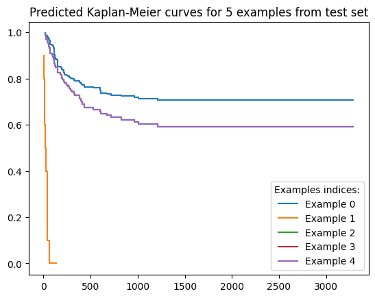
[29]:
for i in range(5):
    plt.step(
        predictions[i]["times"],
        predictions[i]["probabilities"],
        label=f'Example {i}'
    )
plt.legend(title='Examples indices:')
plt.title('Predicted Kaplan-Meier curves for 5 examples from test set')
[29]:
Text(0.5, 1.0, 'Predicted Kaplan-Meier curves for 5 examples from test set')