Example Usage

from imcp import mcp_curve, mcp_score, plot_mcp_curve, imcp_curve, imcp_score, plot_imcp_curve, plot_curve

from sklearn.datasets import load_iris
from sklearn.linear_model import LogisticRegression
from sklearn.ensemble import RandomForestClassifier, GradientBoostingClassifier
from sklearn.svm import SVC

import pandas as pd

MCP curve

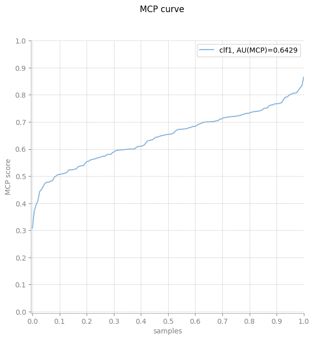
Single MCP curve

X, y = load_iris(return_X_y=True)

clf = LogisticRegression(solver="liblinear").fit(X, y)
probabilities = clf.predict_proba(X)
plot_mcp_curve(y, probabilities)

area = mcp_score(y, probabilities)
print("Area under MCP curve: {:.4f}".format(area))

Area under MCP curve: 0.6429

Multiple MCP curves

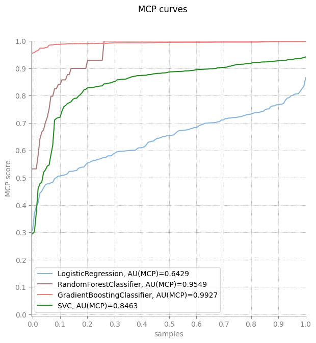
More plots can be drawn on the same figure to make comparison between curves easier. Example below presents curves calculated for different ways of obtaining class probabilities.

X, y = load_iris(return_X_y=True)
algorithms = {'LogisticRegression': LogisticRegression(solver='liblinear'),
             'RandomForestClassifier': RandomForestClassifier(random_state=42),
             'GradientBoostingClassifier': GradientBoostingClassifier(),
             'SVC': SVC(probability=True),}

scores = {}
for key in algorithms:
    algorithms[key].fit(X, y)
    score = algorithms[key].predict_proba(X)
    scores[key] = score
    area = mcp_score(y, score)
    print('Area under MCP curve for {}: {:.4f}'.format(key, area))

plot_mcp_curve(y, scores)

Area under MCP curve for LogisticRegression: 0.6429
Area under MCP curve for RandomForestClassifier: 0.9549
Area under MCP curve for GradientBoostingClassifier: 0.9927
Area under MCP curve for SVC: 0.8463

IMCP curve

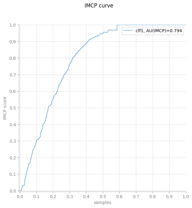
It is also possible to take into account disproportion of class distribution amongst given dataset. In such case, the width of bar for each sample is scaled. Class which covers less samples in the dataset will have wider bars.

There have been implemented analogous methods for all mcp methods - imcp_curve, imcp_score and plot_imcp_curve.

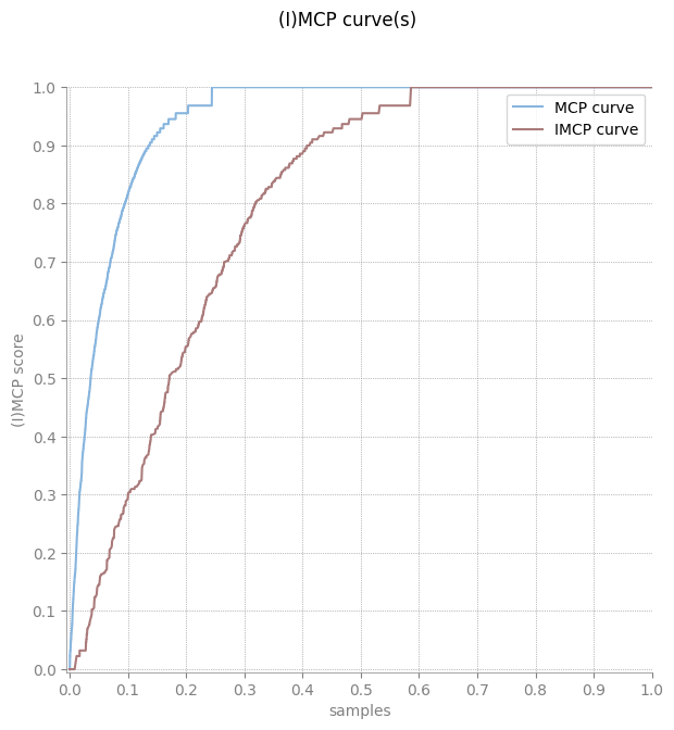
Also, in case that user wants to plot, for example, regular curve and imbalanced curve on the same plot, the plot_curve method has been developed. It allows user to plot any number of curves given as arguments in the same style as plot_mcp_curve and plot_imcp_curve. It is also possible to save figure plot with that method after user has specified output figure path.

df = pd.read_csv('../../../../tests/test_imbalanced_class_probs.csv')

y_true = df["y_true"]
y_score = df.drop(["y_true"], axis=1)

plot_imcp_curve(y_true, y_score, abs_tolerance=0.0000001)

area = imcp_score(y_true, y_score, abs_tolerance=0.0000001)
print("Area under IMCP curve: {:.4f}".format(area))

Area under IMCP curve: 0.7940

Plotting regular MCP and IMCP on the same figure

mcp_x, mcp_y = mcp_curve(y_true, y_score, abs_tolerance=0.0000001)
imcp_x, imcp_y = imcp_curve(y_true, y_score, abs_tolerance=0.0000001)

plot_curve([mcp_x, imcp_x], [mcp_y, imcp_y], label=["MCP curve", "IMCP curve"])